In which I fight my way through decades of legacy and bad habits to find beauty in producing documents with LaTeX.
Motivation
LaTeX is a pain to get started with, not only but mainly because of its legacy going back several decades. Then, you may ask, why do I still prefer it over LibreOffice, Word, you name it? There are compelling reasons ranging from proper kerning to small caps and old style figures. In short: it is still the only viable option for producing visually pleasing documents. For graphical side-by-side comparisons of what this means take a look here and here. In the following I’m going to show you important tricks and hints that helped me find beauty in producing documents with a modern LaTeX approach.
I assume you are somewhat familiar with LaTeX basics. If not, course materials are available here and ShareLaTeX is also quite good.
Building LaTex Documents
To compile a LaTeX document, you invoke the engine The Right Amount Of Times ™. Then bibtex for generating references. Then the LaTeX engine multiple times again to adapt the layout to the inserted references.
Wat? There has to be a better way. And there is!
latexmk
Introducing latexmk: latexmk is similar to make and knows how often and in which order to run the engine and bibtex. It is even able to generate external resources by invoking a makefile itself. I recommend you to take a look at its documentation, as it can be used to fully replace a makefile, with options to wait on changes, trigger rebuilds, and more.
I came to the conclusion that wrapping latexmk in a makefile is still beneficial. Take a look at what my typical LaTeX makefile looks like:
engine="lualatex -interactive=nonstopmode --shell-escape %O %S"
refs = bibliography.bib
sources = main.tex chapters/some-chapters.tex

main.pdf: $(sources)
	@latexmk -pdf -pdflatex=${engine} -bibtex $<

watch:
	@while ! inotifywait --event modify $(refs) $(sources); do make; done

spell:
	@hunspell -l -t -d en_US -i utf-8 $(sources) | sort | uniq --ignore-case

clean:
	@latexmk -C

.PHONY: watch spell clean
This provides you with several targets:
While make builds the document once make watch listens on modifications to your sources and builds the document.
This allows you to keep your document viewer open and get a updated document every time you save your source.
make spell spell checks your sources with hunspell and understands the LaTeX syntax to some degree and make clean delegates to latexmk for removing temporary build files (you probably need to remove some files in addition).
lualatex
I’m using lualatex as an engine.
You may want to replace it with pdflatex or xelatex if you prefer those.
I found lualatex the only viable engine for basically two reasons:
one, it is actively maintained and designed with a modern approach in mind (support for unicode, system fonts, etc.) and two, it does not have ridiculous memory constraints that you easily reach e.g. when plotting charts.
The only downside in using lualatex I found is an increase in build times.
This is a bit frustrating for when using the make watch target and then having to wait multiple seconds until the document gets refreshed in the viewer.
Read the lualatex documentation if you want to make the switch.
Also note that switching to lualatex is not just replacing the engine; you need to switch out a few packages — but all this is documented and is rather easy to do.
In the following I’m assuming you are using lualatex as an engine.
Now that we can build documents let’s take a look at how to design them!
Designing The Document
In the following I’m going to show you how to design your document in a modern approach, making use of some awesome packages.
Document Classes
Document classes describe the document’s purpose: is it a book, a report or even a letter? Unfortunately, there is almost no case for using the ones LaTeX comes with. Instead I recommend the KOMA-Script bundle, that includes modern replacements for LaTeX own document classes. As usual the koma-script documentation is superb — read it!
Switching to the KOMA-Script document classes is as easy as changing your preamble to something along the lines of:
\documentclass[draft=false
             , BCOR=0mm  % correct binding offset when printing
             , 12pt
             , headings=big
             , chapterprefix=true
             , numbers=noenddot]{scrreprt}
Warnings
There is a package that you should include first: nag. Why first? Because it warns you about obsolete commands and package.
\usepackage[l2tabu,orthodox]{nag}
Typography
If you have the time and interest I really recommend you getting The Elements of Typographic Style. A quick introduction is at Butterick’s Practical Typography that is quite good but also opinionated to some degree.
For anything font-related I recommend fontspec. And for improving details you had no idea about, take a look at microtype (with the most beautifully looking documentation)!
\usepackage{fontspec}
\usepackage{microtype}
\frenchspacing
\frenchspacing disables two spaces after a dot, which is what you normally want.
Also read the documentation before adding options; microtype for example is smart enough to do its best in selecting options depending on engine and environment.
In determining which fonts are getting used the pdffonts tool from the poppler-utils package is quite helpful.
Latin Modern is a good default, but I wanted to use Hermann Zapf’s Palatino as main font.
Now is the right time to watch The Art Of Hermann Zapf.
Most good looking fonts that include small caps, old style figures and more, you have to pay for.
Fortunately there is the TeX Gyre project that includes a Palatino remake with TeX Gyre Pagella.
In case you make use of math symbols there is also the recent TeX Gyre Math project.
\usepackage{unicode-math}
\setmainfont[Ligatures=TeX, Numbers=OldStyle]{TeX Gyre Pagella}
\setmathfont{TeX Gyre Pagella Math}
TeX ligatures are e.g. for enabling en-dash and em-dash ligatures. On a related note, learn the difference between a hyphen -, the en-dash – and the em-dash —! Also note that Pagella’s ligatures are ligatures but do not look as fused as in other fonts.
After some research I found sans and mono fonts (that can be scaled automatically to the main font) beautifully matching Palatino:
\setsansfont[Scale=MatchLowercase]{Bitstream Vera Sans}
\setmonofont[Scale=MatchLowercase]{Inconsolata}
Finally, KOMA-Script sets dispositions like \section in bold sans by default.
In my opinion the switch from the main text’s serif font to bold sans is quite distracting.
Instead I’m using serif small caps for dispositions (and the page header) that are not bold by default:
\addtokomafont{disposition}{\rmfamily}
\setkomafont{pagehead}{\scshape}
\setkomafont{disposition}{\scshape}
Language
lualatex works well together with polyglossia — use it instead of babel:
\usepackage{polyglossia}
\setdefaultlanguage{english}
Tables
I found booktabs to produce professional looking tables. Its documentation also gives great hints how to design your table:
\usepackage{booktabs}
Colors
I highly recommend using ColorBrewer for selecting an appropriate color palette:
\usepackage{xcolor}

\definecolor{primary}{RGB}{117,112,179}
\definecolor{secondary}{RGB}{27,158,119}
\definecolor{tertiary}{RGB}{217,95,2}
Source Code
The minted package makes use of Pygments for syntax highlighting. This approach is by far more robust than other listings packages:
\usepackage{minted}
Not to sound like a perfectionist, but there is a way to adapt the color scheme to your document’s color palette. Using the color scheme requires creating and then registering your plugin, which is quite a bit effort.
Plots
I came to the conclusion that native LaTeX graphics just look the best. For this I’m using pgfplots.
What I’m doing is the following:
- save my experiment’s data in an interchangable format, e.g. csv
- load and analyze the data, e.g. with Pandas (save scripts for reproducibility)
- save the processed data in a format that pgfplot understands
- use pgfplots to create beautiful plots
This works great for plot types that are supported by pgfplots (quite a large number, skim the documentation). I also recommend using the units package in addition and setting some sane defaults globally:
\usepackage{tikz}
\usepackage{pgfplots}
\usepgfplotslibrary{units}
\SendSettingsToPgf
\usepgfplotslibrary{statistics}

\pgfplotscreateplotcyclelist{colorscheme}{{primary},{secondary},{tertiary}}

\pgfplotsset{compat=1.11
           , tick label style = {font=\tiny}
	   , % etc.
}
In the following I will show you how to produce a few beautiful looking plots, with negative space as a design decision.
The general idea is to wrap your plot in a figure with htb as placement constraint, i.e. place here, top or bottom but never on a separate page.
In addition you want a caption and a label for all your plots.
\begin{figure}[htb]
  \centering
  \begin{tikzpicture}
    \begin{axis}[options]
      % plot specifics
    \end{axis}
  \end{tikzpicture}
  \caption{My caption}
  \label{fig: my-figure}
\end{figure}
For printing I keep a separate black and white color palette around, as it is hard to find one that is very good for both scenarios. In the following I’m using the color palette from above.
Consult Envisioning Information and The Visual Display of Quantitative Information on visual data representation
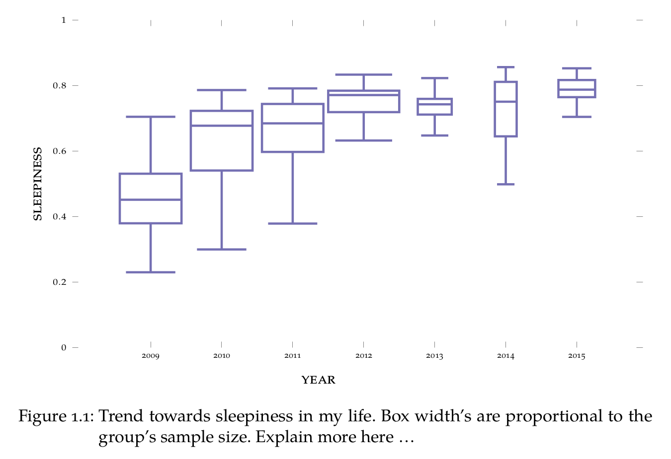
Boxplot
Here’s an example for a boxplot as wide as the main text’s flow and its height respecting the golden ratio for a visually pleasing aspect ratio. The box’s width are also proportional to the group’s sizes — this has to be calculated externally:
\begin{axis}[width=\textwidth
           , height=0.618\textwidth % golden ratio
           , boxplot/draw direction=y
           , xlabel={year}
           , ylabel={sleepiness}
           , ymin=0, ymax=1
           , xtick={1,2,3,4,5,6,7}
           , xticklabels={2009, 2010, 2011, 2012, 2013, 2014, 2015}
           , enlargelimits=0
           , enlarge x limits]
  % box extend is calculated as sqrt(group's size) normalized to [0,1], expressing sample size in boxplot
  \addplot+[boxplot, box extend=0.869] table[row sep=newline,y index=0]{data/boxplot-2009.csv};
  \addplot+[boxplot, box extend=0.869] table[row sep=newline,y index=0]{data/boxplot-2010.csv};
  \addplot+[boxplot, box extend=0.865] table[row sep=newline,y index=0]{data/boxplot-2011.csv};
  \addplot+[boxplot, box extend=1.000] table[row sep=newline,y index=0]{data/boxplot-2012.csv};
  \addplot+[boxplot, box extend=0.478] table[row sep=newline,y index=0]{data/boxplot-2013.csv};
  \addplot+[boxplot, box extend=0.307] table[row sep=newline,y index=0]{data/boxplot-2014.csv};
  \addplot+[boxplot, box extend=0.517] table[row sep=newline,y index=0]{data/boxplot-2015.csv};
\end{axis}
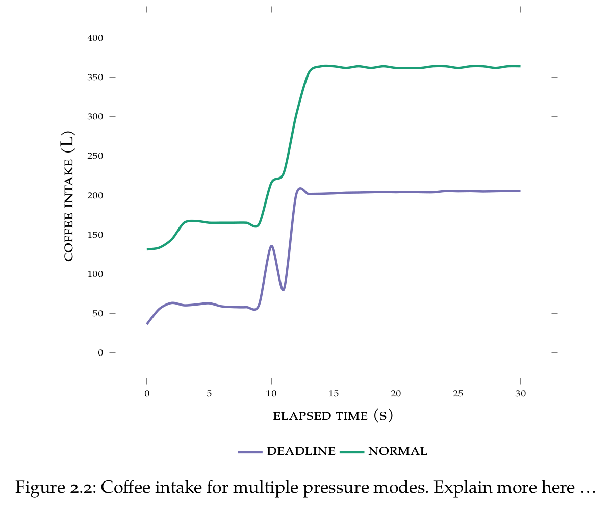
Lineplot
Here’s a trend plot, now only constraining the height to be equal to the golden ratio respecting plots:
\begin{axis}[height=0.681\textwidth,
           , xlabel={elapsed time}
           , ylabel={coffee intake}
           , x unit=\si{\second}
           , y unit=\si{\liter}
           , xmin=0,xmax=30
           , ymin=0,ymax=400
           , smooth]
  \addplot table[x=elapsed,y=intake,col sep=comma]{data/coffee-deadline.csv}; \addlegendentry{deadline};
  \addplot table[x=elapsed,y=intake,col sep=comma]{data/coffee-normal.csv}; \addlegendentry{normal};
\end{axis}
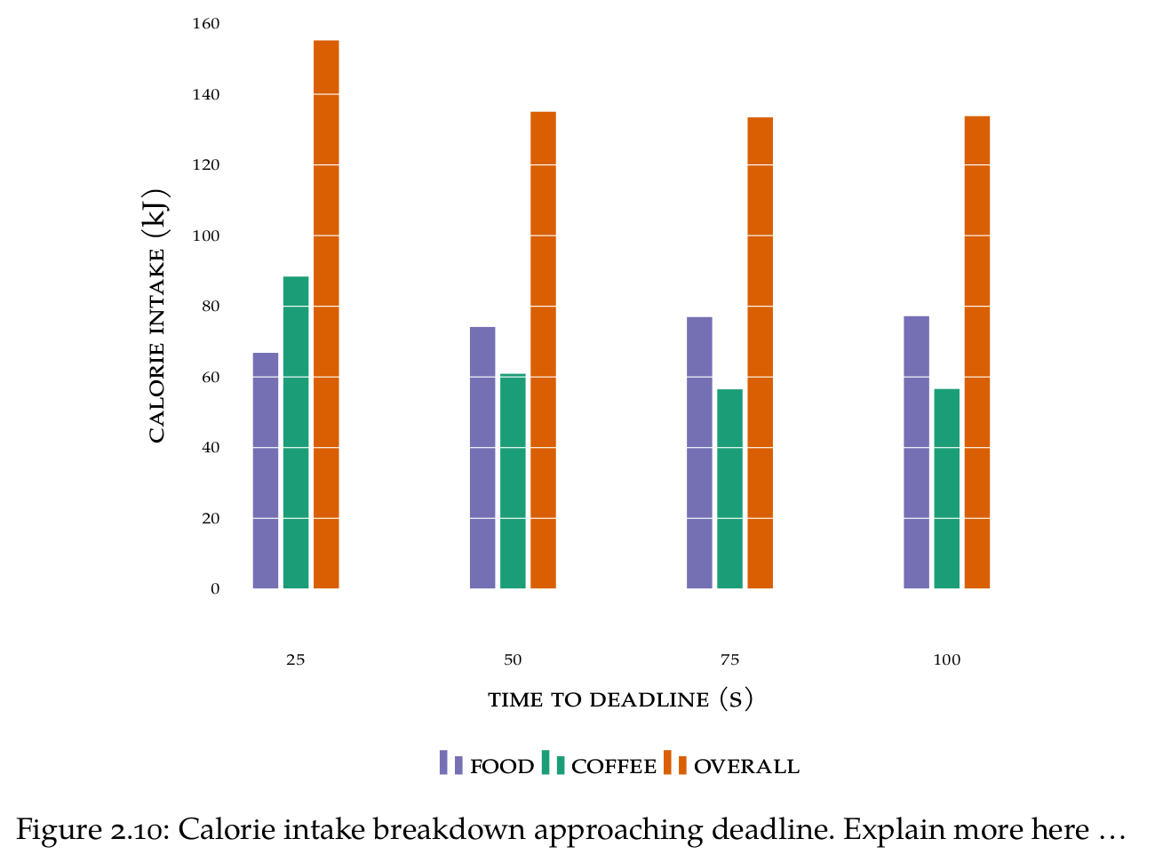
Barplot
And finally a barplot, with the trick of grid lines that are on top and of the same color as the background, as recommended by Edward Tufte:
\begin{axis}[height=0.681\textwidth
           , ybar
           , xlabel={time to deadline}
           , ylabel={calorie intake}
           , x unit=\si{\second}
           , y unit=\si{\joule}
           , change y base
           , y SI prefix=kilo
           , ymajorgrids=true
           , axis on top
           , grid style=white
           , major tick length=0pt
           , ymin=0
           , xtick=data
         ]
  \addplot+[draw opacity=0] table[x=time,y=intake,col sep=comma]{data/intake-food.csv}; \addlegendentry{food}
  \addplot+[draw opacity=0] table[x=time,y=intake,col sep=comma]{data/intake-coffee.csv}; \addlegendentry{coffee}
  \addplot+[draw opacity=0] table[x=time,y=intake,col sep=comma]{data/intake-overall.csv}; \addlegendentry{overall}
\end{axis}
References
I found Biber to be great as a modern BibTeX replacement. There are a few tricks required, e.g. for proper quotes in the references, otherwise it Just Works ™:
\usepackage[strict=true]{csquotes}
\usepackage[backend=biber
          , bibencoding=utf-8
          , safeinputenc
          , bibwarn=true
          , style=alphabetic
          , doi=false
          , isbn=false
          , url=false]{biblatex}
\addbibresource{bibliography.bib}
Scaling
The last trick is to disable print scaling, otherwise your document may be scaled and you absolutely do not want this:
\usepackage{hyperref}
\hypersetup{pdfauthor={My Name}
          , pdftitle={My Title}
          , pdfprintscaling=None}
Markdown
There is a trick that I’m using for writing down notes in markdown and producing a pdf from it. It’s the awesome pandoc tool that is able to convert between a ridiculous amount of formats. For this I have a makefile with a target similar to:
pandoc --filter=pandoc-citeproc --bibliography=$(ref) --toc --latex-engine=$(engine) -o $(target) $(src)